Currently about 1/3rd of the FDA approved drugs are biologics, the vast majority of them being peptides or proteins as well as some oligonucleotides. As biologics are much bigger than small molecule active pharmaceutical ingredients or API’s and can undergo a lot of changes such as deamidation, reduction (or oxidation), covalent modification, etc., the characterization of biologics is much more demanding than of new chemical entities (NCE). Issues like structural changes with regard to folding do normally not occur in small molecule API’s but can cause precipitation or immunological responses with proteins. Also, protein-based biologics may vary depending on the nutrition conditions of the expression system and this needs to be thourougly controlled as otherwise clearance or immunogenicity might vary from batch to batch.
Typical biologics such as monoclonal antibodies have masses in the range of 150 kDa, are heterogeneous and can undergo agglomerisation. Thus the requirements are vastly different for their detection in mass spectrometry in comparison to small molecules such as. e.g. Aspirin or Ibuprofen with masses of a few hundred Dalton. The characterization of protein-based biologics, intact proteins or protein complexes by mass spectrometry often combines various approaches such as peptide-based bottom-up analysis, hydrogen-deuterium exchange or intact protein-based top-down analysis. In particular the latter is often difficult for standard instruments.
The reasons for this are manifold and we will discuss this with several examples and also explain why having a dedicted instrument for intact protein mass spectrometry often makes a lot of sense.
MS Vision is doing active research in the area of native mass spectrometry and high mass MS since its founding in 2004. Originally, this started with modifying quadrupoles to improve transmission and selection at high m/z values. However, it quickly turned out that the quadrupole transmission and selection is only one critical aspect when designing an instrument for native mss spectrometry.
So let’s start from the ions source and go to the detector to explain the components which are to be modified. As a quick introduction, the picture shows a NativeSynapt instrument on the left and a NativeQE on the right side:
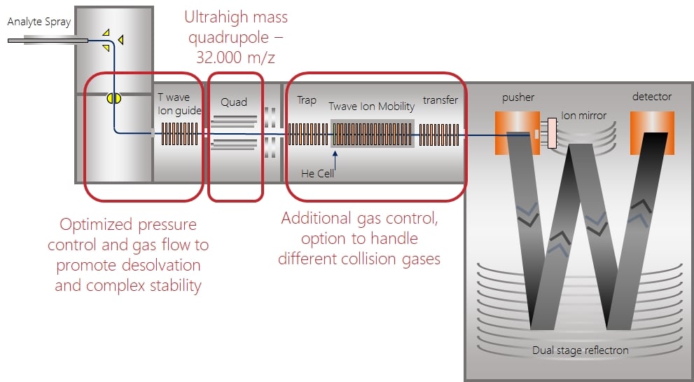
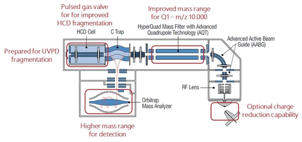
Both systems have in common that the selection quadrupole has been modified as well as the control of the vacuum in the fragmentation region, either the TWave cell in the Synapt or the HCD cell in the QExactive. The source regions of the two systems are pretty different so that they cannot be compared directly.
In the Synapt also the pressure and gas flow in the source has been optimized to promote desolvation and focussing of ions into the instrument. In general, a higher pressure in the beginning of the instrument is beneficial for desolvation as well as for trapping and focussing of ions. However, there are limitations to the pressure as subsequent areas may be affected by increased pressures as well.
The following example shows the effect on ion transmission when the pressure in the StepWave region of a Synapt G2-S(i) instrument is increased:
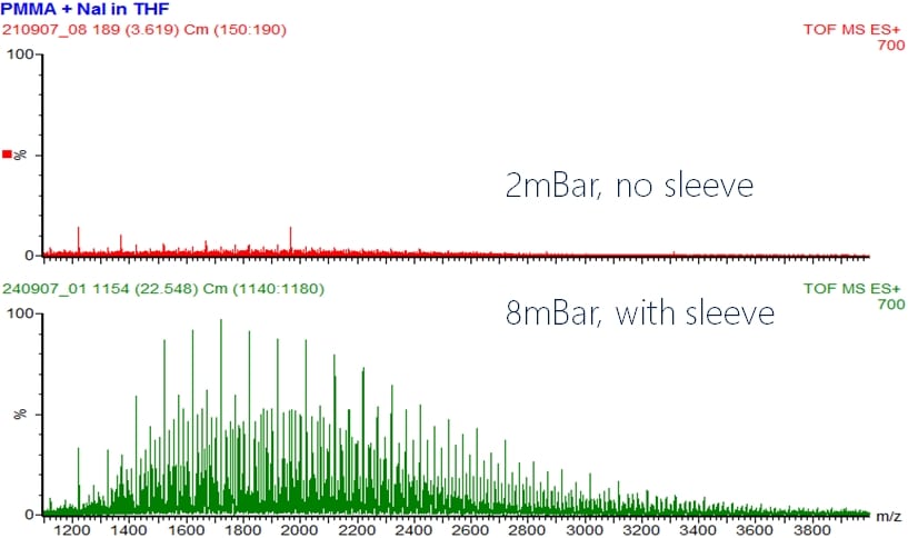
Under otherwise identical conditions, the signal intensity goes from ~15 to 100%, a sixfold increase in transmission. This increase in pressure is also what made the old ABI QStar an excellent instrument for the analysis of intact proteins by mass spectrometry as it also used a sleeve around Q0 while the later TripleTOF systems from Sciex were much less suited for intact proteins or protein complexes due to a change in source design, let alone the maximum quad mass of m/z 1250 for 4600 and 5600 models. But this will be discussed in the following paragraphs.
When these ions then reach the selection quadrupole (Q1 in a QqQ-type system) they want to pass through. Quadrupoles all have similar characteristics, which are determined by the physics behind them. The maximum quad mass (the mass or actually m/z value at which ions travel freely through the quadrupole, the maximum selectable quad mass is also the upper limit of ion selection by the quadrupole) is determined by the potential and the RF-frequency which can be applied. The potential is usually limited by available power supplies, so the easiest is to modify the RF frequency. A standard quadrupole has two modes: Selection or transmission. In the selection mode the quadrupole is operated at a fixed parameter set which allows only a specific m/z value to pass. This is usually used for precursor selection for subsequent fragmentation and represented in the following stability diagram by the blue line as a constant ratio of U/V. For details on what the amplitudes U and V and the later appearing values a and q (which are both proportional to U and V respectively) refer to please see http://www.massspecpro.com/technology/mass-analyzers/quadrupole-mass-filter.
Now let’s have a look at the behaviour of 3 ions with different m/z values, m1 being the largest one, m2 in the middle and m3 as the smallest one. The exact values don’t matter for these consideration.
If m2 is at the quad mass it will be stable and transfer through the quadrupole while the less heavy m3 and the heavier m1 will be unstable and not transmit through the quadrupole.
The dots at the bottom represent the opposite situation where a=0 and many ions are stable (yet not all!). At a given quad mass m2, larger ions will be mostly stable and transmit through the quadrupole while less heavy ions (m3) will quickly reach the limit of the stability diagram and become unstable in x-direction. This is the so-called transmission or RF mode.
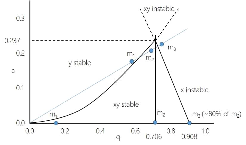
The maximum transmission of a quadrupole is at the so-called “Quad mass” at q=0.706. In RF mode (a=0), the quadrupoles are commonly regarded as total transmission devices. However, that is actually not true, as explained by the stability diagram, they are high pass mass filters (https://www.immun.lth.se/fileadmin/_migrated/content_uploads/TSQtheory_01.pdf) where high masses pass through and transmission drops steeply below around 80% (well, actually it is 0.706/0.908= 77.75%) of the quad mass due to the x-direction instability. When you want to transmit ions from low to high masses, the quad mass needs to be changed (scanned) permanently.
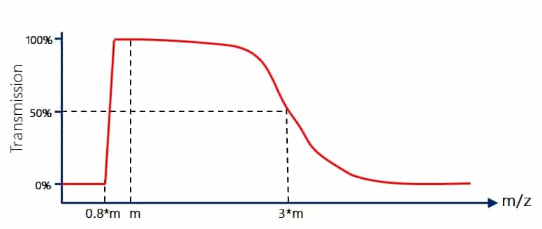
On the higher m/z side the behaviour is slightly different. Here the drop is not steep but has a more sigmoidal shape. The stability diagram would actually predict stability for all heavier ions but other factors come into play here as well. 100% transmission would depend on the fact that the starting point and energy is always well defined and that the movement along the z-axis would be ideal, which is all not the case. Typically, transmission of quadrupoles drops to around 50% at roughly 3 times the quad mass. That means a quadrupole with a maximum quad mass (or upper selection limit) of m/z 2.000 will lose ~50% of the ions at m/z 6.000. This is the reason why for very high m/z values you want large quad masses!
So, when do we need to transfer ions with very high m/z values? The following graph shows the increase of charges with increasing masses of proteins. You can see that for denaturated proteins under acidic conditions the number of charges rises quite quickly with increasing mass, whereas for non-covalent complexes the charge increase is much slower, actually approximately 13 times slower! So as charge increase on denaturated proteins is quick, the m/z values stay low, typically with a maximum at m/z 2.000 or less.
But under native conditions a 400kDa protein or protein complex picks up only around 45 charges and thus has a charge envelope maximum at almost m/z 9.000! That means that with a 2k quadrupole we will already run into a serious ion transmission issue!
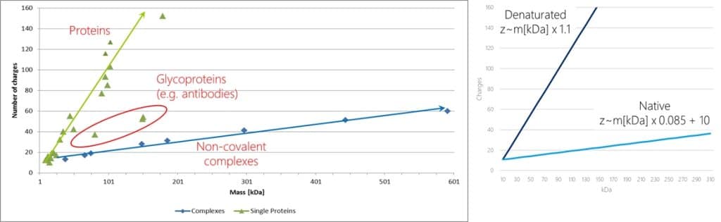
Where does the difference in the charge uptake now come from? Well, we could argue that the difference in the pH of the solution plays a role (denatured proteins are usually analyzed from acidic solutions whereas native MS in most cases is performed using near pH 7 buffered solutions). Probably this plays a role, but the above figure give us an indication of another, much more important contribution: the curve for glycoproteins is between denaturated and native proteins. So they take up less charges as well, even under acidic conditions. Why?
The reason is that the charges in electrospray ionisation sit on the surface of the molecule! Denaturated proteins have a large surface area, often they are unfolded and thus the charge increases almost linearily with the mass. With the chain ejection model for electrospray ion generation (https://www.sciencedirect.com/science/article/abs/pii/S1387380621001585) this can be explained nicely and you can imagine this like a snake crawling out of a droplet being covered with the charges on the surface (think of tipping you finger into oil and pulling it back – it will be covered with oil on the surface!). The chain ejection model explains high numbers of charges on proteins.
With glycoproteins, each N-glycan adds around 2.500-3.500 Da in mass but essentially no place to add charges. Sometimes they even reduce the charges because of acidic sialic acid moieties at the end. Also, the glycan is very flexible and actually covers a huge surface area of the protein. A prominent recent example for this is the SARS-CoV2 spike protein with several glycosylation sites. A comparison on how it looks like with and with glycans is shown here: https://www.maynoothuniversity.ie/research/spotlight-research/unlocking-mysteries-sars-cov-2-sugary-coated-glycan-shield. Almost the entire surface area is covered with the highly flexible glycan chains.
What happens now with native proteins? Under native MS conditions, proteins remain folded and the inner part of the folded proteins is not accessible for protons like the surface for the glycoproteins. Even more, when proteins undergo protein complex assembly, a part of the outer surface is lost as well. Let’s assume our protein is a cube with mass 12.000 Da. On each side of the cube we have one charge. So we end up with a protein which appears at m/z 2.000 (12.000/6) in the mass spectrum. When we now form an octameric complex out of this, we assemble 8 cubes and lose some surface area due to this. Now we have a cube with an outer surface area of 2x2x6=24 which allows for 24 charges. But the mass is now 8×12.000 or 96.000 Da. Thus now we would observe the same molecule in it’s complexed form at m/z 4.000 (96.000/24):
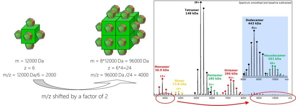
The spectrum shows Alcohol dehydrogenase, a tetrameric protein complex under nativeMS conditions (the higher oligomers can be artifacts because of the protein concentration. Please observe that except of the pentamer, all higher oligomers are multiples of the tetramer). As it can be seen the monomer at 37 kDa has a charge maximum at m/z ~3.000 whereas the octamer has it close to m/z 7.500, a bit more than twice of the monomer. With the curve functions given above an 800 kDa protein would theoretically show up at m/z 11.500 with 70 charges. Let’s see whether that’s true later.
So, under native MS conditions, charge increases much slower than protein or protein complex mass and thus m/z values increase rapidly. Also, here the theory helps us to understand that as under native conditions not the chain ejection model applies but the charge retention model or CRM (see literature above for this). This is the reason why for the analysis of noncovalent protein complexes we need large quadrupoles!
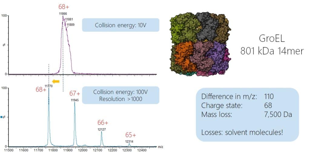
As mentioned before, the desolvation of large molecules is a critical factor for achieving a decent mass spectral signal. The pressure in the source region is one factor to achieve this, the conditions in the collision cell is another one. The following example shows the spectrum of the 800 kDa 14mer complex GroEL. At low collision energy (10V) a broad, unresolved peak is observed. When the collision energy is increased to 100V, still the intact complex is observed (native complexes in MS can handle a lot of collision energy as they can easily dissipate it over the molecule without fragmentation!) but now we see peaks for different charge states and much sharper peaks! When we compare the m/z values and assume they are of identical charge, we observe a mass difference of around 110 Da at 68 charges. This compares to a mass difference of approximately 7.500 Da which mainly consist out of solvent molecules, for water this would correspond to more than 400 water molecules we get rid of! As this “solvation shell” is not homgeneous, this also explains the broad peak as inconsistent numbers of solvent molecules lead to different masses for each protein complex and consequently to broad peaks in the mass spectrum.
As mentioned, native complexes can be very stable under collision conditions and sometimes it is hard to fragment them into monomer units or even induce fragmentation of the protein chains.
To induce the fragmentation to allow to characterize the composition of native complexes we now need to get more energy into the molecules. This can happen by increasing the potential (classically between entrance and exit of the Q2 collision cell which increase the speed with which molecules are dragged through the gas atmosphere in the collision cell). This is limited by the power supplies in the instruments which you usually do not want to exchange because this might change the entire behaviour of the system due to different accuracies, switching delays, etc. But a simple way to increase the energy is using different collsion gases. Mostly, nitrogen (m/z 28) or Argon (m/z 40) is used as collision gas. These gases have similar weight and size. When we now go from there to Xe with m/z 131, the mass of the collision gas is about threefold higher and also the energy which is transferred upon collision with the analyte is much higher. Remember: kinetic energy is E=½mv², thus if the potential and thus the speed is the same, a three times heavier collision gas will transfer three times as much energy than a lighter one!
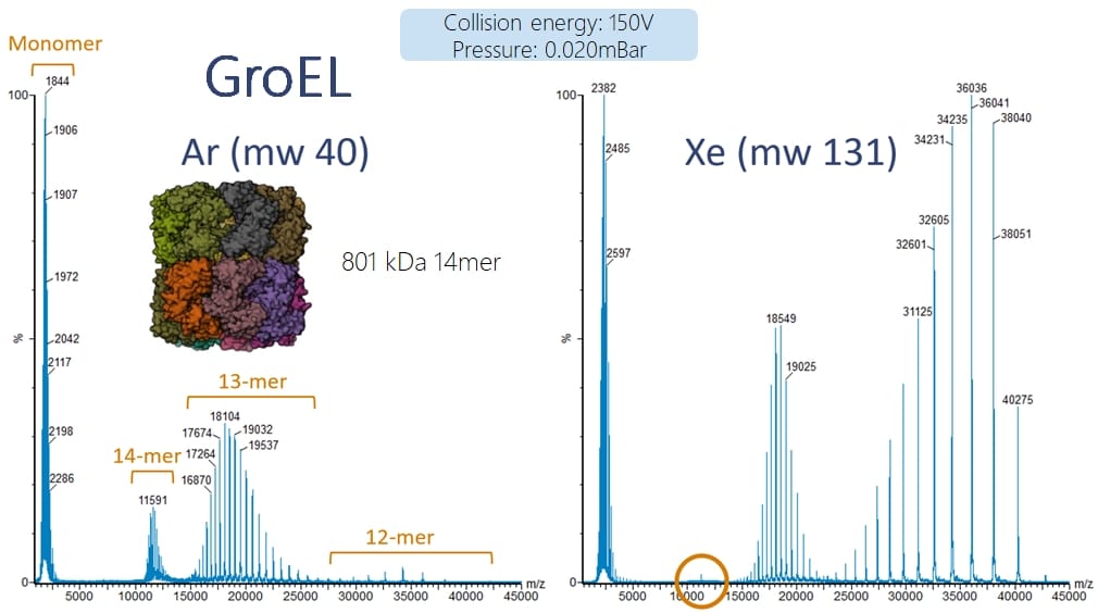
In the example below for the fragmentation of intact GroEL complexes we can see that at the same collision potential (150V) and the same collision gas pressure, with Argon we still see the intact 14mer complex remaining whereas with Xenon we generate much more 12mer and there is almost no 14mer remaining.
Note: above we calculated that an 800 kDa protein complex should appear at ~11.500 with ~70 charges. The GroEL 68+ charge state appears at 11.800 Da and the proteins weight is 801 kDa…
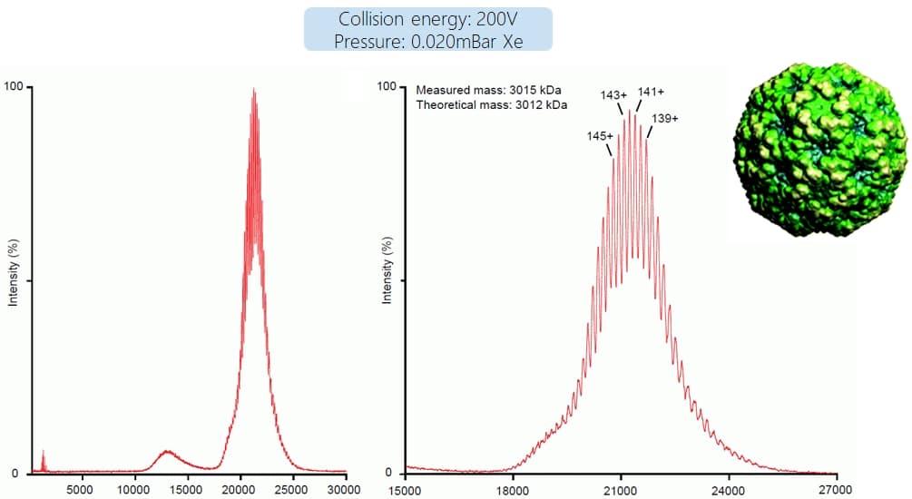
So, we can now – when using the right pressure conditions, collision gases and energies and a decent quadrupole – measure pretty big masses. But how big? The answer is: VERY big. The picture below shows data from an intact 3 MDa virus capsid (data courtesy of Charlotte Uetrecht, CSSB Hamburg). However, we have to admit that this spectrum is a bit exceptional. Not because of the mass, even up to 10 MDa have been successfully measured (https://www.ncbi.nlm.nih.gov/pmc/articles/PMC2938053/pdf/zjw1742.pdf), but because these large molecules are rarely homogenous. And as mentioned before with the solvent shells, heterogeneity causes small mass shifts between individual ion species, leading to peak broadening and as a result a loss of resolution to identify the individual charge states. Therefore, in most cases, for these ultrahigh masses only unresolved peaks are observed and the actual mass has to be inferred by other techniques. But sometimes charge state assignement is still possible!
So, m/z values can be big, masses can be very big. How to detect these now? Since 20 years MS Vision is now modifying TOF based instruments for the detection of these ultrahigh masses. For a normal TOF detector, these m/z values are usually not a problem.
But what we need to keep in mind ist that resolution on TOF systems is limited. Usually in the range between 10.000 and 50.000 for current TOF/QTOF systems. That means we will only observe average peaks when looking at intact proteins as to isotopically resolve the signals, resolution, for baseline separation of peaks, would need to be approximately be at 3x the mass of the protein.
Is a limited resolution critical when doing this type of analysis? No, it is not! And you won’t get much better data anyway! Let’s assume we want to measure a monoclonal antibody of mass 150.000. The figure below shows the calculated signal at an resolution of 10k and 100k (Thanks to David Kilgour from Vibrat-Ion Ltd. for doing the simulations with his AutoVectis software!),
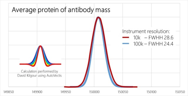
As you can see, the difference is negligible. At both resolution settings we see an unresolved peak, just the full width at half maximum (FWHM) differs slightly. The difference is around 15%, not something which would justify a spending of 2 Mio€ for an FT based instrument instead of 200k€ or less for a TOF based instrument…
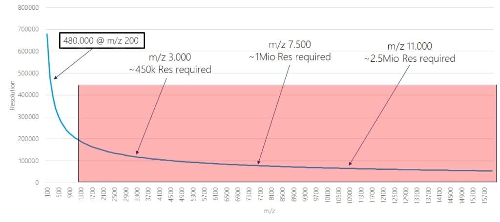
Now, when you think of FT based instruments you might argue that their resolution is much higher, e.g. 480.000, which is more than 3x 150.000. So you can resolve an antibody signal!
Well, actually no. You cannot. The reason is that for FT based acquistions, the resolution drops quickly with increasing m/z values. Resolution is proportional to 1/SQRT(m/z) for Orbitraps and 1/(m/z) for FT-ICR. The figure shows the curve for an Orbitrap based systems specified with a resolution of 480.000 at m/z 200, the drop for FT-ICR is even faster while the starting point is much higher. But the fundamental issue is the same.
If you would like to know which actual (instrument) resolution you can achieve on your Orbitrap system at a given m/z value, you can use our calculator. You can also calculate it by yourself using the following formula:
Resolution=(1/SQRT(m/z))*(Resolution setting*10*SQRT(2))
-
When we now go back to where we observe our protein signals, for an antibody of mass 150kDa we see those at m/z ~3.000 where the remaining resolution is just about 120.000, for higher masses it is even worse. So in no reasonable case on Orbitrap based systems we will observe isotopically resolved spectra for large (e.g. >75-100 kDa) intact proteins, let alone protein complexes. On FT-ICR based systems such measurements have been achieved, but here an additional problem comes into play.
Orbitrap and FT-ICR are both ion trapping systems. If you store many ions of the same charge in a small enclosed space they will repel each other. This is called the “space charge effect”. The space charge effect leads to a significant decrease in spectra quality, loss of mass accuracy and eventually even a complete loss of signal. To control this, trapping mass spectrometry (all of them, also classical ion traps) control the number of trapped ions carefully. You want to have a low number of charges to get good resolution and mass accuracy but you want to have as many as possible to get good sensitivity. Terms for these control mechanisms are e.g. automatic gain control (AGC) at ThermoFisher or ion charge control (ICC) at Bruker.
So what happens with this? Let’s assume we have a monoclonal antibody. This molecule has an isotopic pattern which spans around 70 isotopologues and a dynamic range of around 5 orders of magnitude. That means for a meaningful representation of the isotopic pattern you will need 100.000s of ions to get reasonable ion statistics, each with around 50 charges. An Orbitrap typically can trap around 500.000 charges, that would correspond to 10.000 ions distributed over approximately 30 different charge states and 70 different isotopologes. So with every scan we have 30×70=2100 individual species, each with on average 5 ions on which we want to represent 5 orders of magnitude of dynamic range. That is almost impossible. If we look at data of isotopically resolved antibody spectra (e.g. https://www.ncbi.nlm.nih.gov/pmc/articles/PMC3215840/pdf/nihms333487.pdf) we see exactly this issue of very bad ion statistics. So, even if you can resolve the signals isotopically, the result is only of an academic value. The practical value is almost zero as you cannot reasonably fit theoretical isotopic patterns into the data.
Another phenomenon is based on the FT-based detection in Orbitraps and ICR and is called “beat structure”. Essentially it results from an overlay of many closely related frequencies as they occur from many isotopologues of the same charge state of a protein (see https://pubs.acs.org/doi/abs/10.1021/jasms.1c00336# for further details). It occurs in both techniques and the resulting signal basically shows a number of equally spaced signals like heartbeats in an ECG. The signal intensity drops over time because of signal dispersion and the important thing is that the information is only in the beats, everything between those is only noise.
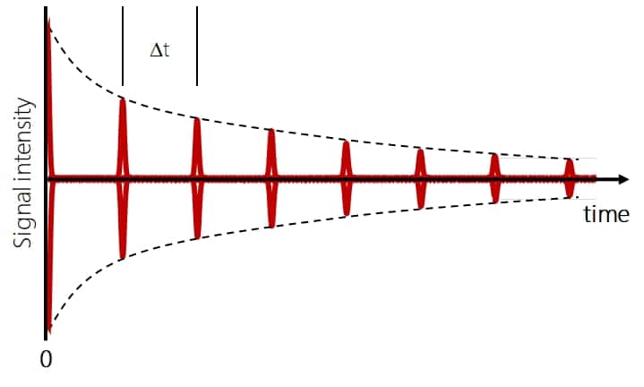
The distance Δt between the beats depends on the mass of the protein and the charge. The larger the protein mass and the lower the charge, the larger is Δt (https://pubs.acs.org/doi/10.1016/j.jasms.2009.03.024). E.g. for the 40+ charge state of the 80 kDa protein Transferrin in a classic (not high field) Orbitrap analyzer, the distance between the beats is already ~1 sec. But to get good resolution, mass accuracy and signal intensity you need at least 1-2 beats in addition to the initial beat (the initial one at 0 sec is mandatory to get any signal at all), the more the better. At least in older Orbitrap analyzer models the FID acquisition time was limited to 2 seconds and that made intact protein analysis very difficult.
So when we have all these technical challenges, why should we modify an Orbitrap based system such as QExactive for high mass and native MS at all?
Well, the reason is that their resolution for low to medium masses is still excellent and you can do both, peptide-based bottom up analysis and intact protein work on the same system. And as many of these system are already out in the field and meanwhile fully deprectiated and being replaced by newer generation systems, these systems can be upgraded for relatively low costs to give aditional information and value which makes nativeMS much more affordable then by buying new high end systems. Another factor is that upgrades for biologics analysis on ThermoFisher QExactive systems were only available with the original purchase of the system, not retrospecively. That means customers which did not decide for this option during the purchase cannot upgrade the systems later with the original ThermoFisher Biopharma upgrade. The MS Vision NativeQE upgrade enables this and also provides larger mass ranges for selection and detection in comparison to the ThermoFisher Biopharma upgrade as well as improved HCD fragmentation performance.
All this brought us to the conclusion that, while we genuinely think that TOF like in our NativeSynapt is the detector of choice for ultralarge intact proteins and protein complexes, a high mass optimized QExactive has its place nevertheless as NativeQE in biopharma and biologics characterization workflows.
For an independent, yet contentwise very similar, review article from Iain D.G. Campuzano and Joseph A. Loo please refer to “Evolution of Mass Spectrometers for High m/z Biological Ion Formation, Transmission, Analysis and Detection: A Personal Perspective” published in JASMS (https://doi.org/10.1021/jasms.4c00348).